by Ruth Mottram and Peter Langen
Glaciers in Greenland lose mass by melt and runoff, by calving and by submarine melt that happens at the front of outlet glaciers that terminate in the ocean. Submarine melt occurs because the ocean water is (relatively) warmer than the ice, but it goes much faster where there is turbulent water mixing the layers by the glacier. Probably the most important source of turbulence are plumes of water that emerge at the base of the glacier where it terminates in the fjord. The water is generated by melting mostly at the surface though also at the bed of the glacier. Meltwater flows like rivers through systems of englacial channels to finally arrive at the bed where it makes its way, eventually, to the end of the glacier.
Unfortunately these channels are pretty hard to map, and there are lakes and areas at the bed where water can be stored. The plumes themselves are rather hazardous to observe as they are often inaccessible and in front of actively calving sections of the glacier. There have been a few studies, but often these are snapshots in time and it is difficult to assess how important these processes are to the overall mass budget of the ice sheet.
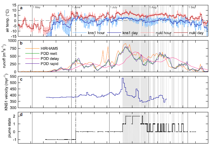
Therefore we have to turn to models to work out how important plume processes are for submarine melt. In our recent paper with Slater et al (2017), we contributed data from the HIRHAM5 RCM to look at runoff within a catchment in Greenland. The case study was based at Kangiata Nunata Sermia glacier, in the Godthåbsfjord area of south western Greenland. It’s a relatively accessible glacier showing many of the common processes for Greenland outlet glaciers and has a fair bit of data available. The Langen et al (2014) paper showed that HIRHAM5 performs pretty well in terms of modelled runoff in this region.
The modelled runoff was used in two different models of subglacial plumes, including one implemented in MITgcm, in order to determine what configuration of subglacial hydrology and plume distribution along the ice front was most likely. The models were compared with a time lapse photos of the ice front showing plume activity at the surface.
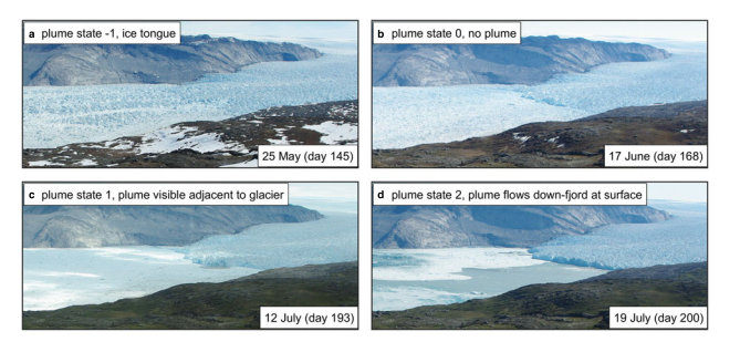
For a large proportion of the summer, the modelled catchment runoff greatly exceeds the discharge required to create a plume that would reach the fjord surface, yet there are extended periods when there is no plume visible from the time lapse pictures. This can only be explained by the runoff emerging into the fjord in a spatially distributed fashion. In the paper we therefore argue that subglacial drainage near the glacier terminus is often spatially distributed, formed either from numerous point sources of subglacial discharge, or a single but very wide subglacial channel or possibly a complex combination of the two.
There are two implications from this work. Firstly, a more spatially distributed submarine plume gives a higher total melt than a single concentrated plume but this melt rate is still unable to explain the mass loss at the terminus when considering the ice velocity at the terminus, suggesting that calving is still the most important mass flux term at this glacier. Secondly, the modelling study found that the distributed hydrology, suggested by the results leads to a more direct ice flow response to high surface melt rates and this response most likely scales with catchment size.
Probably the most important result to come out of this study is that longer time series of observations of plumes, in combination with the modelled runoff lead to a dramatically different understanding of key processes within the fjords when compared to those suggested by simple snapshot observations in earlier studies.