Martin Olesen successfully defended his thesis at the University of Copenhagen Monday 18th February. The thesis is entitled “High resolution climate simulation. Methods for improving and customising climate information with focus on outreach and uncertainty assessment”. His supervisors has been Jens H. Christensen, Peter Lang Langen and Eigil Kaas. The assessment committee consisting of Aslak Grinsted, Niels Bohr Institute, KU. Prof. Dr. Daniela Jacob, GERICS, Institute Helmholtz-Zentrum Geesthacht and Research Prof. Tim Carter, Finnish Environment Institute.

You Can read the abstract at the Niels Bohr Institute webpage

Henrik Sadatzki successfully defended his thesis for the PhD degree at the University of Bergen. The thesis is entitled: “Sea ice variability in the Nordic Seas over Dansgaard–Oeschger climate cycles during the last glacial – A biomarker approach”

 

Ice2ice Phd Mads Bruun Poulsen the 16/01-2019 successfully defended his PhD thesis on Parameterizing Southern Ocean eddy-induced circulation in coarse resolution ocean models. He was evaluated by an impressed committee consisting of Professor, Brian Vinter, eScience, Niels Bohr Institute, University of Copenhagen, Associate Professor, David Ferreira, Department of Meteorology, University of Reading, and Professor Joe LaCasce, Department of Geosciences, University of Oslo. He has been supervised by Markus Jochum from the Niels Bohr Institute.

Abstract: Baroclinic mesoscale eddies in the Southern Ocean induce a circulation which modulates wind-driven ventilation of the interior ocean, with implication for exchanges of heat and carbon dioxide with the atmosphere. In coarse resolution ocean general circulation models which do not explicitly resolve mesoscale eddies, eddy-induced circulation is typically parameterized with a skew-diffusive tracer flux that depends on an eddy transfer coefficient, κ. Several plausible closures for κ exist, yet consensus on a specific expression for κ remains largely absent in the ocean modeling community and results in uncertain Southern Ocean ventilation rate estimates. With the use of two ocean general circulation models of coarse and eddy-resolving horizontal resolution, this thesis assesses the properties of two recently proposed expressions for κ with the aim to provide guidance towards the optimal closure.

First an expression for κ which solely depends on local stratification is examined in a suite of model simulations with varying intensity of the zonal wind stress in the Southern Ocean. The simulations suggest that implementation of a dynamic κ alleviates coarse models from an overly sensitive overturning circulation although the parameterized eddy-induced circulation does not completely match that found in the eddy-resolving model. The latter shortcoming is associated with an overly strong poleward eddy heat transport in the coarse model, which is largely compensated by mean-flow heat transports. In addition, the coarse model demonstrates a centennial equilibration time scale to wind stress change that, if representative of the dynamics, has implication for evaluation of eddy compensation in eddying models.

Second, an expression for κ which additionally depends on eddy geometry and energy is investigated. It is shown that this closure derives from a correspondence between horizontal eddy buoyancy fluxes and variance ellipses, which offers a concise geometric interpretation of baroclinic mean-flow stability and vertical momentum transfers. The eddy geometry is examined in the eddy-resolving model to assess its potential to form basis for parameterization. The geometry obeys simple probability distributions and is insensitive to external forcing change, but also possesses vertical structure which relates to the orientation of horizontal eddy buoyancy fluxes with respect to the large-scale buoyancy gradient. This structure is not explained by rotational fluxes and hence represents a possible parameterization challenge.

The thesis also presents estimates of κ extracted directly from the eddy-resolving model and provides a discussion on the assumption of horizontally down-gradient eddy fluxes upon which the skew-diffusive tracer flux relies. In particular, this discussion reiterates a previous finding that a dynamically important component of the horizontal eddy buoyancy flux appears unaccounted for in coarse models.

During the annual Norwegian Geological Society winter conference held in Bergen this week Eystein Jansen was today awarded the Brøgger prize. The prize is the highest mark of honor a geologist can be given in Norway and is awarded to persons “…that have contributed in a unique way to understand especially the geology of Norway or geology in general” as written in the prize statutes.

The list of Eystein’s important scientific contributions given by the jury is very impressive; first the establishment of the Laboratory for geological mass spectronomy in Bergen in 1983, then the establishment and leadership in the Bjerknes Center for Climate Research (CoE) for 13 years starting in year 2000, his involvement in the establishment of the SapienCE – Centre for early human behavior (another CoE) in 2017, his contribution to the IPCC report and not at least his decisive role for the understanding the ocean circulation in the North Atlantic and link to the variation of ice sheets during the ice ages.

The fact that he has brought together geologists and modellers to better understand the climate system (as in Ice2ice) is also mentioned as an important contribution by the jury.

Congratulations Eystein!

You can read about Eystein and the award here, unfortunately only in Norwegian.

by Joel Pedro

In the climate system, like the ecosystem, everything is connected. Arctic terns migrate each year from their Arctic breeding grounds to the Antarctic coast. Our recent paper in Nature shows that a similar 50,000 km journey is made by abrupt Dansgaard-Oeschger (DO) climate change events.

The specific new result is that each Dansgaard-Oeschger event is accompanied—within a few decades—by a pulse of Antarctic warming and a northward shift in the westerly winds that circle the continent. Similarly, when the DO events abruptly end we see a pulse of Antarctic cooling and the westerlies shift back north.

The speed at which the southern temperature and wind changes occur implies that, like the terns, they make their way to Antarctica through the atmosphere. The rapid atmospheric changes are superimposed on more gradual (and already well-documented) changes in Antarctic temperature that appear around 200 years later and that are attributed to changes in ocean heat transport and mixing.

To stretch the bird analogy, the terns return north after their foray in the Antarctic sea ice, and similarly Antarctica is not the last stop for the DO signal. The next step is to test whether the wind changes are an important component in driving the next DO event, e.g. through their effects on the overturning circulation, air-sea carbon fluxes and sea ice.

Why the southern westerlies shift with the DO events is not yet fully understood, but model studies suggest a plausible chain of events that matches observations (see our ice2ice paper from earlier this year on this topic): abrupt warming in the Arctic means that the thermal equator is displaced north and the SH Hadley cell strengthens; the stronger SH Hadley cell redistributes energy back into the cooler southern hemisphere, in turn strengthening the sub-tropical jet and drawing the westerlies northward. The resulting Antarctic temperature changes are consistent with the observed influence of the Southern Annular Mode on Antarctic climate, suggesting similar atmospheric dynamics may be involved.

In its details, our study examined ice cores from five different locations around Antarctica and synchronized their dating internally using layers of volcanic ash. Changes in the temperature and in the source regions of Antarctic snowfall were then analysed by looking at water isotope ratios. Credit is due to Christo Buizert (OSU) who led the study and to Bradley Markle, who published similar findings in 2017 that were restricted to the Pacific sector of Antarctica.

Last week a new ice2ice article was published-below the ice2ice authors have written a short version covering the main findings. The full paper can be found here: Geng, Marilena Sophie, Jens Hesselbjerg Hesselbjerg Christensen, and Torben Christensen. “Potential future methane emission hot spots in Greenland.” Environmental Research Letters (2018).

by Marilena Sophie Geng, Jens Christensen Hesselbjerg, and Torben Røjle Christensen

Permafrost is defined as ground at a soil temperature below freezing for at least two consecutive years.  It is an important part of the cryosphere as 25 % of the northern hemisphere is underlain by permafrost and it stores a large amount of carbon in the frozen ground.

In a changing climate and warming Arctic, permafrost is starting to thaw more and more. The frozen organic matter in the ground can therefore reach temperatures above freezing and become available to decay. Decomposition of organic matter produces greenhouse gases. A feedback loop is triggered, higher temperatures lead to thawing permafrost lead to greenhouse gas emission lead to higher temperatures. Depending on the oxygen available to decay either carbon dioxide (CO2) or methane (CH4, which we concentrated our work on) is released.

Permafrost can be found in all cold regions like Alaska, northern Canada, Siberia and Greenland. As we had high spatial resolution model simulations of Greenland (figure 1) for present and future scenarios at hand, we used those for a permafrost analysis.

The issue with permafrost analysis is that most climate models don’t have permafrost and methane emissions included in their formulation. A high resolution of the soil and complicated processes within it (that are partially still not fully understood) would be needed which is often computationally to expensive at the moment. So our idea was to find a way to derive permafrost conditions and methane emissions from parameters that are in all climate models.

In a first step we use an established frost index that uses a ratio of degree days of freezing and thawing to derive permafrost conditions from our HIRHAM5 regional climate simulations. We can compare the permafrost conditions predicted by the frost index with observations from Greenland. As we are satisfied with the performance of the frost index and the model, we use the index for simulations of future climate scenarios and find spots on Greenland that showed significant thawing of permafrost (figure 2).

In a second step, we need to find a correlation between methane emissions from permafrost and some other variable included in the climate model. We can use methane flux data from the GEM (Greenland ecosystem monitoring) project in Nuuk and Zackenberg. We test correlations of methane emissions with air temperature, sensible and latent heat flux. Finally, we find that an exponential relationship between methane emissions and air temperature describe the observations best. As the air temperature rises, methane CH4 emissions increase exponentially.

We can use the found correlation all over Greenland with our present day and future simulated temperatures. When we now compare our maps of future potential methane emissions and permafrost thaw we find spots that show both, potential high emissions and thawing permafrost (figure 2 and 3). These spots, like Kangerlussuaq and Scoresby land, are likely to show high emission in the future and need some additional monitoring.

Congratulations to ice2ice PhD Nicholas Rathmann at Centre for Ice and Climate who successfully defended his PhD thesis Monday 26 November 2018, and obtained the degree of Doctor of Philosophy. Nicholas will continue to work as Postdoc at the Centre for Ice and Climate.

Title and abstract of the PhD thesis:

Title: “Nonlinear fluid dynamics – Studies on the dynamics of ice sheet deformation and the turbulent energy cascade”

Abstract: Nonlinear fluid motion occurs naturally in central components of the climate system. Studying such motion is instrumental for improving the accuracy and realism of models of climate components, which has important implications for future climate projections. This thesis presents four studies on the topic of nonlinear fluid dynamics addressing two subjects: the dynamics of ice sheet deformation and the dynamics of the turbulent energy cascade.

The first study investigates the controlling mechanisms of the observed 2016 seasonal speed-up of Zachariae and Nioghalvfjerdsfjorden outlet glaciers in northeast Greenland, which drain a significant part of the Greenland ice sheet. From surface imagery made available by the newest generation of satellites, state-of-theart velocity maps are derived, and the timings of processes potentially impacting the speed-up are estimated. By combining observations with numerical modelling, it is shown that the subglacial environment exerts an important control over the ice discharge rate of the region, which has implications for estimating the region’s contribution to near-term sea level rise.

The second study investigates the influence of strong single-maximum fabrics on the transient deformation of internal layers within ice sheets. By using a new Lagrangian numerical ice flow model, it is shown that discrete, strong single maximum layers — which may account for suppressed shearing along nonbasal crystallographic planes — are a plausible candidate for explaining the disturbed flow observed from ice-penetrating radar transects. The results have potential implications for interpreting ice-core stratigraphies and chronologies, as well as understanding of how internal disturbances might influence surrounding flow fields.

The third and fourth study address the origin of the transfer direction of kinetic energy between scales of motion (upscale/downscale) in fully developed turbulence using the spectral-helical decomposition of the velocity field. In this decomposition, the nonlinear term in the Navier–Stokes equation becomes to a sum over eight distinct types of three-wave interactions. In the third study, a simple model (a shell model) is introduced to investigate the behaviour of the eight types of nonlinear interactions, which is compared to a linear stability analysis, finding a fair agreement. In the fourth study, a subset of the three-wave interactions are shown to conserve a new positive-definite quadratic quantity in addition to kinetic energy, which cause the interactions to contribute to a reverse transfer of energy in three dimensions (small to large scales) in analogy to two-dimensional turbulence. Understanding the energy transfer directionality, and possible ties between two- and three-dimensional turbulence, has implications for geophysical flows such as the free atmosphere and oceans where vertical motion in many places is suppressed, thereby affecting predictability time scales and the transport of energy and momentum in climate.

by ice2ice PhD Andreas Plach

Many people are interested in how much the melting of the Greenland ice sheet will contribute to rising sea levels in the future. In my PhD I therefore investigate how the Greenland ice sheet looked like during the last period with much warmer summers on Greenland than today, a period called the Eemian interglacial period approximately 125,000 years ago. Ice from this period has been found in several Greenland ice cores and we therefore know that Eemian ice is preserved at the bottom of the Greenland ice sheet. Unfortunately, it is impossible to get an exact picture of the Eemian ice sheet from these few ice core data points and we therefore need to use computer models to simulate the Eemian ice sheet and get a more complete picture of its extent and the sea level rise it caused. If we know how much smaller the Eemian Greenland ice sheet was, this will help us to know how the Greenland ice sheet behaves in a warmer climate and to estimate how much smaller it will become in the warming future.

However, it is challenging to simulate the Eemian Greenland ice sheet. Many previous studies which did simulate the Eemian ice sheet, got very different results (Fig. 1). In our recent paper, we try to understand what caused the large differences in between these previous studies and we focus on how different surface mass balance (SMB) models (which are used to simulate the melting of the ice sheet) behave in the warm Eemian climate. A comparison of various SMB (melt) models shows large differences in melt between these models. Since the previous studies (Fig. 1) partly used different SMB models, the variation in simulated melt in these SMB models is likely a cause for the differences between the previous studies. Our results show the high importance of SMB model selection for Eemian ice sheet simulations which will help scientists to improve future attempts to simulate the Eemian Greenland ice sheet.

Want to know more?

Read the full paper where we compare different surface mass balance (SMB) models for the Eemian interglacial period: https://www.clim-past.net/14/1463/2018/cp-14-1463-2018.pdf

You might also be interested in our recent discussion paper where we simulate the Eemian Greenland ice sheet with a selection of SMBs derived in the paper above: https://www.the-cryosphere-discuss.net/tc-2018-225/tc-2018-225.pdf

 

 

 

The following ice2ice article was recently published: Sessford, E. G., et al. “High resolution benthic Mg/Ca temperature record of the intermediate water in the Denmark Strait across D‐O stadial‐interstadial cycles.” Paleoceanography and Paleoclimatology (2018). Below ice2ice Evangeline Sessford has written about the findings. This blogpost also appears on http://www.scisnack.com/

 

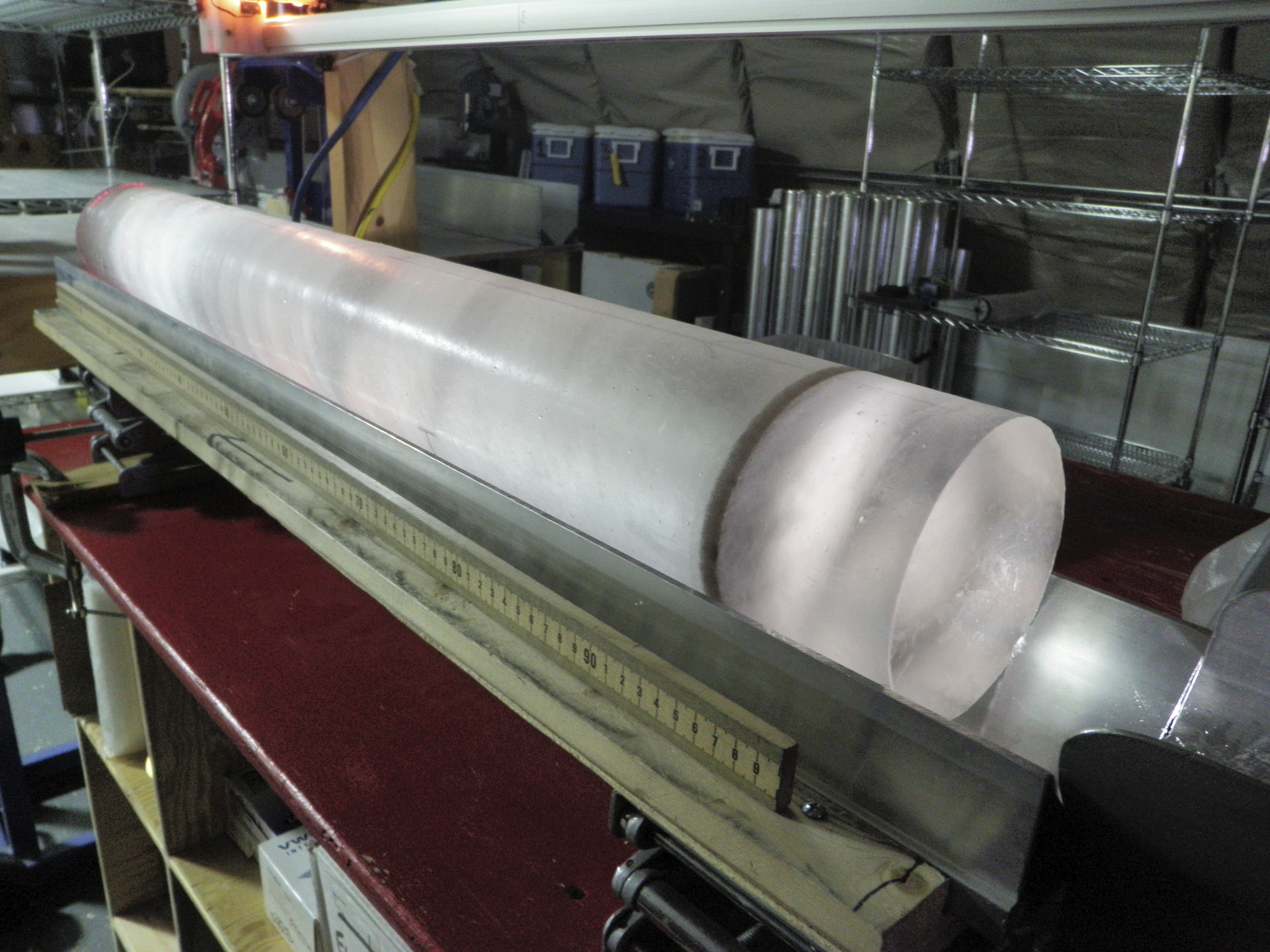
We set sail from Iceland on Research Vessel G.O. Sars, in July 2015, to extract sediment cores from the ocean floor in the Denmark Strait. The aim was to find sediment containing fossilized shells of zooplankton called foraminifera, to aid our understanding of what the past ocean was like. Over time, mud and foraminifera shells accumulate layer by layer, year after year building the ocean floor. These separate layers contain valuable information about how the ocean climate system changed over time in the past because the oldest layers are at the bottom. We cannot measure the past directly therefore we need proxies.

Proxies are substitute measurements that reflect ocean properties in the past. For example, to get a record of past ocean temperatures we measure the amounts of magnesium and calcium in foraminifera shells. These amounts depend on ocean water temperature. The higher the magnesium to calcium ratio; the higher the temperature. One of the cores, GS15-198-36CC -or Caprice, as I like to call her- was exceptionally full of our required proxy.

We measured the magnesium to calcium ratio in the shells of a type of foraminifera that lives on the ocean floor. Caprice was extracted from 770m below the surface so the measurements reflect intermediate depth water masses and how they changed over time.

Different water masses in the ocean have different characteristics. For example, the modern Gulf Stream flowing into the Nordic Seas at the surface in the east is warm and saline Atlantic Water. However, as it circulates in the Nordic Seas it loses heat to the atmosphere, cools and sinks and returns to the North Atlantic through the Denmark Strait in the west as intermediate water.

Some warm Atlantic Water makes it up to the Arctic Ocean. The Arctic Ocean is covered with sea ice and a cool, fresh layer of water. This water is lighter than the warmer Atlantic Water. Despite being warmer, the Atlantic Water is forced below the fresh layer because of its higher salt content and therefore density. This warm intermediate water then circulates in the Arctic Ocean while retaining most of its heat content and exits as intermediate water with a similar temperature as it entered.

The measurements from Caprice indicate that both these processes happened at our core location in the Denmark Strait during the last ice age, 30-40 thousand years ago. Basically, our core indicates that the Nordic Seas were sometimes covered by sea-ice and were sometimes open.

Results from Caprice record an intermediate water mass in the Denmark Strait that alternated between periods of cold (-1 to 1 °C), fluctuating and warm (1 to 3 °C), stable temperatures. These large shifts in the intermediate water temperature record are coherent with substantial, well-known climate fluctuations, Dansgaard-Oeschger events. These events are clearly visible in Greenland ice core records that show air temperatures rapidly warming by up to 15 °C in less than 30 years. The abrupt warmings and following warm periods are known as Greenland Interstadials. They were followed by drops back into cold periods known as Greenland Stadials. Research suggests that these shifts between interstadials and stadials are governed by a fluctuating sea ice cover retreating and then expanding over most of the Nordic Seas.

Our magnesium-calcium proxy measurements support this timeline of events. When the intermediate water was warm and stable -similar to the modern-day Arctic Ocean- there was sea ice cover over the Nordic Seas and it was a Greenland Stadial. When the intermediate water was cold and fluctuating -similar to modern Nordic Seas- there was no sea ice cover over the Nordic Seas, and it was a Greenland Interstadial.

Our measurements of intermediate water from Caprice help us understand what happened with sea ice at the surface of the Nordic Seas thousands of years ago. But we are still left wondering how the ocean actually circulated during these events.  The stories from cores like Caprice become truly spellbinding when you combine them with other scientific methods, like modelling. Only then can we get a complete picture of how the oceans behaved. We need to extend the study area from where we were on board G.O. Sars to the inflow region in the eastern Nordic Seas. We will incorporate a model to test if the ocean was physically capable of these proposed fluctuations.

 

References:

• Dansgaard, W., et al. (1993), Evidence for general instability of past climate from a 250-kyr ice-core record, Nature, 364, 218-220.
• Rahmstorf, S. (2002), Ocean circulation and climate during the past 120,000 years, Nature, 419, 207-214.
• Rosenthal, Y., and B. K. Linsley (2007), Mg/Ca and Sr/Ca paleothermometry, in Paleoceanography, Physcial and Chemical Proxies, pp. 1723-1731.
• Rudels, B., G. Björk, J. Nilsson, P. Winsor, I. Lake, and C. Nohr (2005), The interaction between waters from the Arctic Ocean and the Nordic Seas north of Fram Strait and along the East Greenland Current: results from the Arctic Ocean-02 Oden expedition, Journal of Marine Systems, 55(1–2), 1-30.
• Voelker, A. (2002), Global distribution of centennial-scale records for Marine Isotope Stag (MIS) 3: a database, Quaternary Science Reviews, 21, 1185-1212.

Check out the links below if you’re craving to learn more about the ocean:

Movies:

More about proxies – https://vimeo.com/154733972

More about Dansgaard-Oeschger events – https://vimeo.com/156830900

 

For kids and teaching:

https://climatekids.nasa.gov/ocean/

https://iglo.w.uib.no/

Recently the ice2ice article Risebrobakken, Bjørg, and Sarah Miche Patricia Berben. “Early Holocene establishment of the Barents Sea Arctic front.” Frontiers in Earth Science 6 (2018): 166 was published in Frontiers Earth Science. You can find the full article here. Below a short summary by the two ice2ice authors Bjørg Risebrobakken and Sarah M. P. Berben from Uni Research Climate, Bjerknes Centre for Climate Research, Bergen, Norway and Department of Earth Science, University of Bergen, Bjerknes Centre for Climate Research, Bergen, Norway, respectively.

 

by Bjørg Risebrobakken and Sarah M. P. Berben

A main feature of the Barents Sea oceanography is the Arctic front. The Arctic front marks the transition between the dominating water masses of the Barents Sea: Atlantic Water in the south and Arctic Water in the north. Presently, the Barents Sea Arctic front is directed by the topography of the Bear Island Trough and to some degree the location of the sea ice boundary.

During the last glacial maximum, the Svalbard-Barents Sea and Scandinavian Ice Sheets covered the Barents Sea. Hence, no water entered the Barents Sea, neither from the south nor from the north. Following the deglaciation of the Barents Sea, the present-day ocean circulation developed. The evolution of how the present location of the Barents Sea Arctic front established during the early Holocene is documented by foraminiferal relative assemblage data from six core sites along the western Barents Sea margin and opening. The relative abundance of Arctic front indicator Turborotalita quinqueloba, in combination with the cold, polar Neogloboquadrina pachyderma and warm, Atlantic Neogloboquadrina incompta, are used to infer the location of the Barents Sea Arctic front relative to the individual core sites.

 

 

Until ca. 11 ka BP, the Barents Sea Arctic front followed the western margin of the Barents Sea. All sites along the Barents Sea margin where still dominated by Arctic Water between ca. 11 and 10.2 ka BP, however, the Barents Sea Arctic front turned eastwards into the southwestern Barents Sea.

From ca. 10.2 to 8.8 ka BP, the Barents Sea Arctic front moved eastward and was located right above most sites as it followed the Barents Sea margin. The northwestern Barents Sea Arctic front was close to the present location from ca. 8.8 to 7.4 ka BP, however, it was still confined to the southwestern Barents Sea.

From ca. 7.4 ka BP, the Barents Sea Arctic front has been located close to the present position, along the margin southwards from Svalbard, turning eastwards along and beyond the northern Bear Island Trough margin.